Ring Resonator
Ring Resonator
Ring Resonantor
Source Code
1
2
3
4
5
6
7
import gplugins.modes as gmode
import numpy as np
import matplotlib.pyplot as plt
import meep as mp
import gdsfactory as gf
import gplugins.gmeep as gm
import gdsfactory.cross_section as xs
1
2
Using MPI version 4.1, 1 processes
[32m2025-10-12 00:27:25.505[0m | [1mINFO [0m | [36mgplugins.gmeep[0m:[36m<module>[0m:[36m39[0m - [1mMeep '1.31.0' installed at ['/home/ramprakash/anaconda3/envs/si_photo/lib/python3.13/site-packages/meep'][0m
Ring Resonator from gdsfactory
Source Code
1
2
3
4
5
6
7
8
9
10
11
12
13
14
15
16
17
18
19
20
21
22
my_cross_section = xs.strip(width=0.5, radius=10)
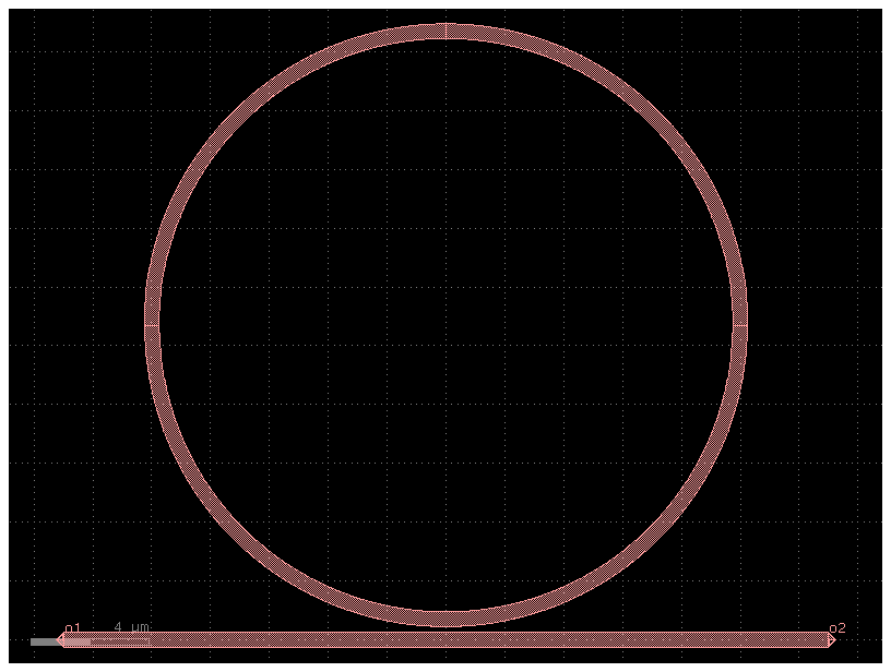
ring_resonator_single = gf.components.ring_single(
gap=0.2,
# radius=100,
length_x=0,
length_y=0,
cross_section=my_cross_section,
bend=gf.components.bend_circular,
)
ring_resonator_single.draw_ports()
ring_resonator_single.plot()
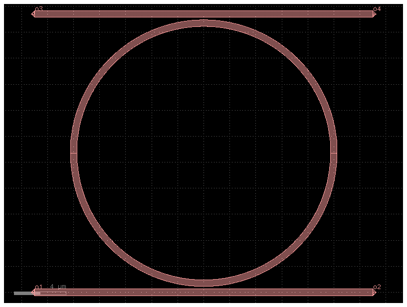
ring_resonator_double = gf.components.ring_double(
gap=0.2,
# radius=10,
length_x=0,
length_y=0,
cross_section=my_cross_section,
bend=gf.components.bend_circular,
)
ring_resonator_double.draw_ports()
ring_resonator_double.plot()
1
2
/home/ramprakash/anaconda3/envs/si_photo/lib/python3.13/site-packages/gdsfactory/components/couplers/coupler90.py:42: UserWarning: {'radius': 10.0} ignored for cross_section 'strip'
  x = gf.get_cross_section(cross_section, radius=radius)

Source Code
1
2
scene = ring_resonator_double.to_3d()
scene.show()
S-paramter for all pass ring resonator.
Optimized for resonace at 1.55um
Analytical discriprion
Resonace:
$L = 2\pi R$
$\beta L = m2\pi$; $\beta = \frac{2\pi n}{\lambda}$
Let, $\lambda=1.55 \mu m$, then
$m=\frac{2\pi R n_{eff}}{\lambda}$
Source Code
1
2
3
4
5
6
7
8
9
10
11
12
13
14
15
16
17
18
19
20
21
22
23
24
25
26
27
28
29
30
31
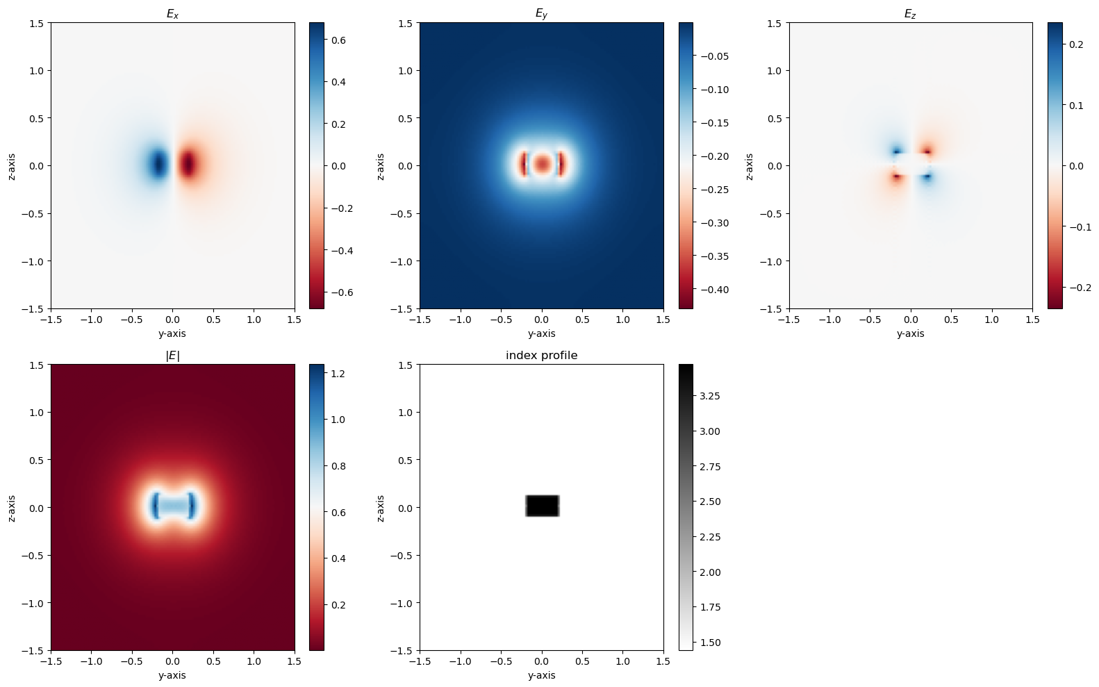
# Calcualte neff and group index using mode solver from gplugins
modes = gmode.find_modes_waveguide(
parity=mp.NO_PARITY,
core_width=0.4,
core_material=3.47,
clad_material=1.44,
core_thickness=0.22,
resolution=40,
sy=3,
sz=3,
nmodes=4,
)
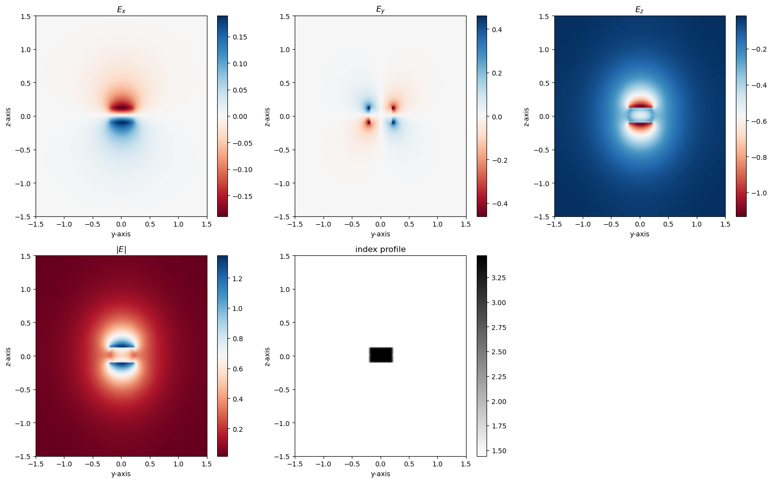
m1 = modes[1]
m2 = modes[2]
m3 = modes[3]
m1.plot_e_all()
m2.plot_e_all()
print("Effective index of mode 1 = ", m1.neff)
print("Effective index of mode 2 = ", m2.neff)
# Calcualting the group index
disp = gmode.find_mode_dispersion(
wavelength=1.55,
wavelength_step = 0.01,
core='Si',
clad='SiO2',
mode_number=1
)
print('The group index =', disp.ng)
1
2
3
Effective index of mode 1 =  2.212251105731657
Effective index of mode 2 =  1.6813883197157091
The group index = 4.276256881279943
Source Code
1
2
3
4
5
6
7
8
9
10
11
R = 10 # Radius of the ring
lam = 1.55
neff = m1.neff # effective index of mode 1
ng = disp.ng # Group index
mode_num = 2*np.pi*R*neff/lam # mode number

# Free spectral range (FSR)
FSR = lam**2/(2*np.pi*R*ng)

print('mode number = ', mode_num)
print('Free spectral range =', FSR,'um')
1
2
mode number =  89.67731382790285
Free spectral range = 0.008941692732543 um
Meep simulation
Source Code
1
2
3
4
5
6
7
8
9
10
11
12
13
14
15
16
17
18
19
20
21
22
23
24
25
26
27
28
29
30
31
32
33
34
35
36
37
38
39
40
41
42
43
44
45
46
47
48
49
50
51
52
53
54
55
56
57
58
59
60
61
62
63
64
65
66
67
68
69
70
71
72
73
74
75
76
77
78
79
80
81
82
83
84
85
86
87
88
89
90
91
92
93
94
95
96
97
98
99
100
101
102
103
104
105
106
107
108
109
110
111
112
113
114
115
116
117
118
119
120
121
122
123
124
125
126
127
128
129
130
131
132
133
134
135
136
137
138
139
140
141
142
143
144
145
146
147
148
149
150
151
152
153
154
155
156
157
158
159
160
161
162
163
164
%%writefile Ring_MPI_sim.py
import gplugins.modes as gmode
import numpy as np
import matplotlib.pyplot as plt
import meep as mp
import gdsfactory as gf
import gplugins.gmeep as gm
import gdsfactory.cross_section as xs

# mp.verbosity(0)

my_cross_section = xs.strip(width=0.5, radius=10)
ring_resonator_single = gf.components.ring_single(
    gap=0.1,
    # radius=100,
    length_x=0,
    length_y=0,
    cross_section=my_cross_section,
    bend=gf.components.bend_circular,
)

# Set up frequency points for simulation
npoints = 10000
lcen = 1.55
dlam = 0.03
wl = np.linspace(lcen - dlam / 2, lcen + dlam / 2, npoints)
fcen = 1 / lcen
fwidth = 3 * dlam / lcen**2
fpoints = 1 / wl

# Center frequency mode_parity
mode_parity = mp.EVEN_Y + mp.ODD_Z
dpml = 1
dpad = 1
resolution = 30

# Define materials
Si = mp.Medium(index=3.45)
SiO2 = mp.Medium(index=1.45)

# Cell size
cell_size = mp.Vector3(ring_resonator_single.xsize + 2 * dpml, ring_resonator_single.ysize + 2 * dpml + 2 * dpad, 0)

# Create the ring resonator component
ring_resonator_single = gf.components.extend_ports(ring_resonator_single, port_names=["o1", "o2"], length=2)
ring_resonator_single = ring_resonator_single.copy()
ring_resonator_single.flatten()
ring_resonator_single.center = (0, 0)

# Get geometry from component
geometry = gm.get_meep_geometry.get_meep_geometry_from_component(ring_resonator_single)

geometry = [
    mp.Prism(geom.vertices, geom.height, geom.axis, geom.center, material=Si)
    for geom in geometry
]
# Source
src = mp.GaussianSource(frequency=fcen, fwidth=fwidth)
source = [
    mp.EigenModeSource(
        src=src,
        eig_band=1,
        eig_parity=mode_parity,
        eig_kpoint=mp.Vector3(1, 0, 0),
        direction=mp.NO_DIRECTION,
        size=mp.Vector3(0, 1),
        center=mp.Vector3(ring_resonator_single.ports["o1"].x + dpml + 2, ring_resonator_single.ports["o1"].y),
        amplitude=1
    ),
]

# Simulation
sim = mp.Simulation(
    resolution=resolution,
    cell_size=cell_size,
    boundary_layers=[mp.PML(dpml)],
    sources=source,
    geometry=geometry,
    default_material=SiO2,
    # symmetries=[mp.Mirror(mp.Y)]
)

# Mode monitors
m1 = mp.Volume(
    center=mp.Vector3(ring_resonator_single.ports["o1"].x + dpml + 2 + 0.5, ring_resonator_single.ports["o1"].y),
    size=mp.Vector3(0, 1),
)
m2 = mp.Volume(
    center=mp.Vector3(ring_resonator_single.ports["o2"].x - dpml - 1 - 0.5, ring_resonator_single.ports["o2"].y),
    size=mp.Vector3(0, 1),
)

mode_monitor_1 = sim.add_mode_monitor(fpoints, mp.ModeRegion(volume=m1))
mode_monitor_2 = sim.add_mode_monitor(fpoints, mp.ModeRegion(volume=m2))
whole_dft = sim.add_dft_fields([mp.Ez], 0.6489713803621261, 0, 1, center=mp.Vector3(), size=cell_size)

# Only plot from master process
if mp.am_master():
    print(f"Running simulation with {mp.count_processors()} MPI processes...")
    sim.plot2D(labels=False)
    plt.savefig('simulation_geometry.png', dpi=150, bbox_inches='tight')
    plt.close()

# Run simulation
# sim.run(
#         until_after_sources=mp.stop_when_fields_decayed(
#             25, mp.Ez, 1e-2
#         )
#     )
sim.run(
    mp.at_every(2000, lambda sim: print(f"Time: {sim.meep_time():.1f}")),
    until_after_sources=mp.stop_when_dft_decayed(tol=1e-9, maximum_run_time=10000)
)

# Calculate S parameters
norm_mode_coeff = sim.get_eigenmode_coefficients(
    mode_monitor_1, [1], eig_parity=mode_parity
).alpha[0, :, 0]

port1_coeff = (
    sim.get_eigenmode_coefficients(mode_monitor_1, [1], eig_parity=mode_parity).alpha[0, :, 1]
    / norm_mode_coeff
)

port2_coeff = (
    sim.get_eigenmode_coefficients(mode_monitor_2, [1], eig_parity=mode_parity).alpha[0, :, 0]
    / norm_mode_coeff
)

# Get field data
eps_data = sim.get_epsilon()
ez_data = sim.get_dft_array(whole_dft, mp.Ez, 0)

# Save results (only from master process)
if mp.am_master():
    np.save('wavelengths.npy', wl)
    np.save('port1_coeff.npy', port1_coeff)
    np.save('port2_coeff.npy', port2_coeff)
    np.save('eps_data.npy', eps_data)
    np.save('ez_data.npy', ez_data)

    # Create field plot
    fig = plt.figure(figsize=(12, 8))
    ax_field = fig.add_subplot(1, 1, 1)
    ax_field.set_title("Steady State Fields")
    ax_field.imshow(
        np.flipud(np.transpose(eps_data)),
        interpolation="spline36",
        cmap="binary"
    )

    ax_field.imshow(
        np.flipud(np.transpose(np.real(ez_data))),
        interpolation="spline36",
        cmap="RdBu",
        alpha=0.9,
    )
    ax_field.axis("off")
    plt.savefig('steady_state_fields.png', dpi=150, bbox_inches='tight')
    plt.close()

    print("Simulation completed successfully!")
    print(f"Results saved to: wavelengths.npy, port1_coeff.npy, port2_coeff.npy, eps_data.npy, ez_data.npy")
    print(f"Plots saved to: simulation_geometry.png, steady_state_fields.png")
1
Overwriting Ring_MPI_sim.py
Source Code
1
!mpirun -np 24 python Ring_MPI_sim.py
Source Code
1
2
3
4
5
6
7
8
9
10
11
12
13
14
15
16
17
18
19
20
21
22
23
24
25
26
27
28
29
30
31
32
33
34
35
36
37
38
39
40
41
42
43
44
45
46
# Load results
wl = np.load('wavelengths.npy')
port1_coeff = np.load('port1_coeff.npy')
port2_coeff = np.load('port2_coeff.npy')
eps_data = np.load('eps_data.npy')
ez_data = np.load('ez_data.npy')
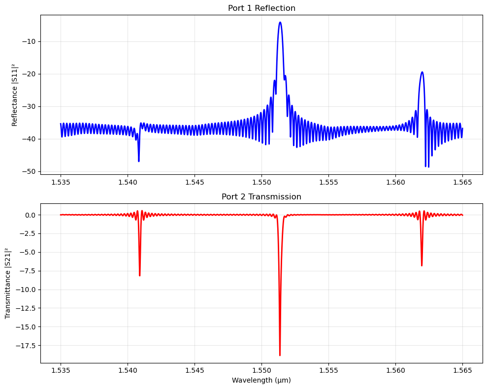
# Plot transmission spectrum
fig, (ax1, ax2) = plt.subplots(2, 1, figsize=(10, 8))
# S11 (reflection)
ax1.plot(wl, 10*np.log10(np.abs(port1_coeff)**2), 'b-', linewidth=2)
ax1.set_ylabel('Reflectance |S11|²')
ax1.set_title('Port 1 Reflection')
ax1.grid(True, alpha=0.3)
# S21 (transmission)
ax2.plot(wl, 10*np.log10(np.abs(port2_coeff)**2), 'r-', linewidth=2)
ax2.set_xlabel('Wavelength (μm)')
ax2.set_ylabel('Transmittance |S21|²')
ax2.set_title('Port 2 Transmission')
ax2.grid(True, alpha=0.3)
plt.tight_layout()
# plt.savefig('transmission_spectrum.png', dpi=150, bbox_inches='tight')
plt.show()
print(f"Peak transmission: {np.min(np.abs(port2_coeff)**2):.4f}")
print(f"Resonance wavelength: {wl[np.argmin(np.abs(port2_coeff)**2)]:.4f} μm")
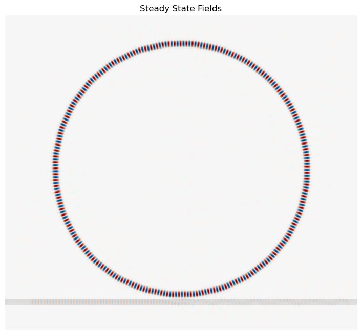
fig = plt.figure(figsize=(12, 8))
ax_field = fig.add_subplot(1, 1, 1)
ax_field.set_title("Steady State Fields")
ax_field.imshow(
np.flipud(np.transpose(eps_data)),
interpolation="spline36",
cmap="binary")
ax_field.imshow(
np.flipud(np.transpose(np.real(ez_data))),
interpolation="spline36",
cmap="RdBu",
alpha=0.9,
)
ax_field.axis("off")
plt.show()
1
Resonance wavelength: 1.5514 μm
FSR from MEEP FDTD
Source Code
1
2
3
4
# index of the the resonaces
index = np.argsort(10*np.log10(np.abs(port2_coeff)**2))[:3]
FSR = wl[index[1]]-wl[index[2]]
print('FSR from meep', np.abs(FSR))
1
FSR from meep 6.000600059952177e-06
Double ring resonator
Source Code
1
2
3
4
5
6
7
8
9
10
11
12
13
14
15
16
17
18
19
20
21
22
23
24
25
26
27
28
29
30
31
32
33
34
35
36
37
38
39
40
41
42
43
44
45
46
47
48
49
50
51
52
53
54
55
56
57
58
59
60
61
62
63
64
65
66
67
68
69
70
71
72
73
74
75
76
77
78
79
80
81
82
83
84
85
86
87
88
89
90
91
92
93
94
95
96
97
98
99
100
101
102
103
104
105
106
107
108
109
110
111
112
113
114
115
116
117
118
119
120
121
122
123
124
125
126
127
128
129
130
131
132
133
134
135
136
137
138
139
140
141
142
143
144
145
146
147
148
149
150
151
152
153
154
155
156
157
158
159
160
161
162
163
164
165
166
167
168
169
170
171
172
173
174
175
176
177
178
179
180
181
182
183
%%writefile RingDob_MPI_sim.py
import gplugins.modes as gmode
import numpy as np
import matplotlib.pyplot as plt
import meep as mp
import gdsfactory as gf
import gplugins.gmeep as gm
import gdsfactory.cross_section as xs

# mp.verbosity(0)

my_cross_section = xs.strip(width=0.5, radius=10)
ring_resonator_double = gf.components.ring_double(
    gap=0.1,
    # radius=100,
    length_x=0,
    length_y=0,
    cross_section=my_cross_section,
    bend=gf.components.bend_circular,
)

# Set up frequency points for simulation
npoints = 10000
lcen = 1.55
dlam = 0.03
wl = np.linspace(lcen - dlam / 2, lcen + dlam / 2, npoints)
fcen = 1 / lcen
fwidth = 3 * dlam / lcen**2
fpoints = 1 / wl

# Center frequency mode_parity
mode_parity = mp.EVEN_Y + mp.ODD_Z
dpml = 1
dpad = 1
resolution = 30

# Define materials
Si = mp.Medium(index=3.45)
SiO2 = mp.Medium(index=1.45)

# Cell size
cell_size = mp.Vector3(ring_resonator_double.xsize + 2 * dpml, ring_resonator_double.ysize + 2 * dpml + 2 * dpad, 0)

# Create the ring resonator component
ring_resonator_double = gf.components.extend_ports(ring_resonator_double, port_names=["o1", "o2", "o3","o4"], length=2)
ring_resonator_double = ring_resonator_double.copy()
ring_resonator_double.flatten()
ring_resonator_double.center = (0, 0)

# Get geometry from component
geometry = gm.get_meep_geometry.get_meep_geometry_from_component(ring_resonator_double)

geometry = [
    mp.Prism(geom.vertices, geom.height, geom.axis, geom.center, material=Si)
    for geom in geometry
]
# Source
src = mp.GaussianSource(frequency=fcen, fwidth=fwidth)
source = [
    mp.EigenModeSource(
        src=src,
        eig_band=1,
        eig_parity=mode_parity,
        eig_kpoint=mp.Vector3(1, 0, 0),
        direction=mp.NO_DIRECTION,
        size=mp.Vector3(0, 1),
        center=mp.Vector3(ring_resonator_double.ports["o1"].x + dpml + 2, ring_resonator_double.ports["o1"].y),
        amplitude=1
    ),
]

# Simulation
sim = mp.Simulation(
    resolution=resolution,
    cell_size=cell_size,
    boundary_layers=[mp.PML(dpml)],
    sources=source,
    geometry=geometry,
    default_material=SiO2,
    # symmetries=[mp.Mirror(mp.Y)]
)

# Mode monitors
m1 = mp.Volume(
    center=mp.Vector3(ring_resonator_double.ports["o1"].x + dpml + 2 + 0.5, ring_resonator_double.ports["o1"].y),
    size=mp.Vector3(0, 1),
)
m2 = mp.Volume(
    center=mp.Vector3(ring_resonator_double.ports["o2"].x - dpml - 1 - 0.5, ring_resonator_double.ports["o2"].y),
    size=mp.Vector3(0, 1),
)
m3 = mp.Volume(
    center=mp.Vector3(ring_resonator_double.ports["o3"].x + dpml + 2 + 0.5, ring_resonator_double.ports["o3"].y),
    size=mp.Vector3(0, 1),
)
m4 = mp.Volume(
    center=mp.Vector3(ring_resonator_double.ports["o4"].x - dpml - 1 - 0.5, ring_resonator_double.ports["o4"].y),
    size=mp.Vector3(0, 1),
)
mode_monitor_1 = sim.add_mode_monitor(fpoints, mp.ModeRegion(volume=m1))
mode_monitor_2 = sim.add_mode_monitor(fpoints, mp.ModeRegion(volume=m2))
mode_monitor_3 = sim.add_mode_monitor(fpoints, mp.ModeRegion(volume=m3))
mode_monitor_4 = sim.add_mode_monitor(fpoints, mp.ModeRegion(volume=m4))
whole_dft = sim.add_dft_fields([mp.Ez], 0.6402048655569782, 0, 1, center=mp.Vector3(), size=cell_size)

# Only plot from master process
if mp.am_master():
    print(f"Running simulation with {mp.count_processors()} MPI processes...")
    sim.plot2D(labels=False)
    plt.savefig('RingDob_simulation_geometry.png', dpi=150, bbox_inches='tight')
    plt.close()

# Run simulation
# sim.run(
#         until_after_sources=mp.stop_when_fields_decayed(
#             25, mp.Ez, 1e-2
#         )
#     )
sim.run(
    mp.at_every(2000, lambda sim: print(f"Time: {sim.meep_time():.1f}")),
    until_after_sources=mp.stop_when_dft_decayed(tol=1e-9, maximum_run_time=5000)
)

# Calculate S parameters
norm_mode_coeff = sim.get_eigenmode_coefficients(
    mode_monitor_1, [1], eig_parity=mode_parity
).alpha[0, :, 0]

port1_coeff = (
    sim.get_eigenmode_coefficients(mode_monitor_1, [1], eig_parity=mode_parity).alpha[0, :, 1]
    / norm_mode_coeff
)

port2_coeff = (
    sim.get_eigenmode_coefficients(mode_monitor_2, [1], eig_parity=mode_parity).alpha[0, :, 0]
    / norm_mode_coeff
)

port3_coeff = (
    sim.get_eigenmode_coefficients(mode_monitor_3, [1], eig_parity=mode_parity).alpha[0, :, 1]
    / norm_mode_coeff
)
port4_coeff = (
    sim.get_eigenmode_coefficients(mode_monitor_4, [1], eig_parity=mode_parity).alpha[0, :, 0]
    / norm_mode_coeff
)

# Get field data
eps_data = sim.get_epsilon()
ez_data = sim.get_dft_array(whole_dft, mp.Ez, 0)

# Save results (only from master process)
if mp.am_master():
    np.save('RingDob_wavelengths.npy', wl)
    np.save('RingDob_port1_coeff.npy', port1_coeff)
    np.save('RingDob_port2_coeff.npy', port2_coeff)
    np.save('RingDob_port3_coeff.npy', port3_coeff)
    np.save('RingDob_port4_coeff.npy', port4_coeff)
    np.save('RingDob_eps_data.npy', eps_data)
    np.save('RingDob_ez_data.npy', ez_data)

    # Create field plot
    fig = plt.figure(figsize=(12, 8))
    ax_field = fig.add_subplot(1, 1, 1)
    ax_field.set_title("Steady State Fields")
    ax_field.imshow(
        np.flipud(np.transpose(eps_data)),
        interpolation="spline36",
        cmap="binary"
    )
    ax_field.imshow(
        np.flipud(np.transpose(np.real(ez_data))),
        interpolation="spline36",
        cmap="RdBu",
        alpha=0.9,
    )
    ax_field.axis("off")
    plt.savefig('RingDob_steady_state_fields_.png', dpi=150, bbox_inches='tight')
    plt.close()

    print("Simulation completed successfully!")
    print(f"Results saved to: RingDob_wavelengths.npy, RingDob_port1_coeff.npy, RingDob_port2_coeff.npy, RingDob_eps_data.npy, RingDob_ez_data.npy")
    print(f"Plots saved to: simulation_geometry.png, steady_state_fields.png")
1
Overwriting RingDob_MPI_sim.py
Source Code
1
2
# Cell 3: Run with MPI
!mpirun -np 24 python RingDob_MPI_sim.py
Source Code
1
2
3
4
5
6
7
8
9
10
11
12
13
14
15
16
17
18
19
20
21
22
23
24
25
26
27
28
29
30
31
32
33
34
35
36
37
38
39
40
41
42
43
44
45
46
47
48
49
50
51
52
53
54
55
56
57
58
59
60
61
62
63
64
import numpy as np
import matplotlib.pyplot as plt
# Load results
wl = np.load('RingDob_wavelengths.npy')
port1_coeff = np.load('RingDob_port1_coeff.npy')
port2_coeff = np.load('RingDob_port2_coeff.npy')
port3_coeff = np.load('RingDob_port3_coeff.npy')
port4_coeff = np.load('RingDob_port4_coeff.npy')
eps_data = np.load('RingDob_eps_data.npy')
ez_data = np.load('RingDob_ez_data.npy')
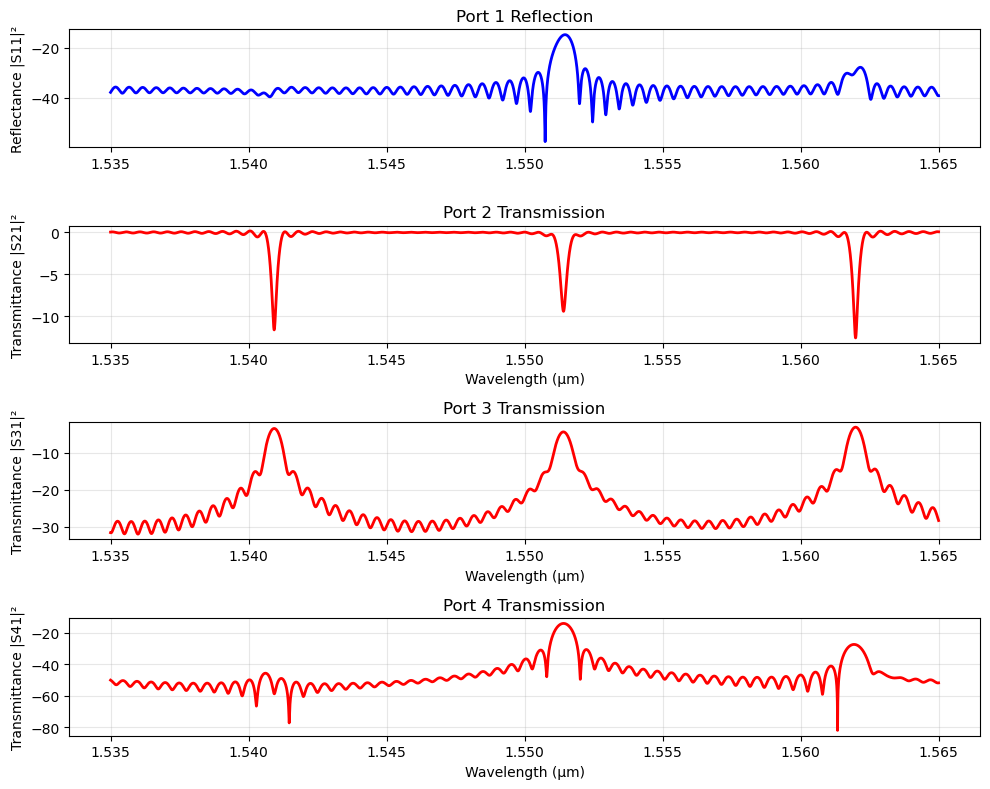
# Plot transmission spectrum
fig, (ax1, ax2, ax3, ax4) = plt.subplots(4, 1, figsize=(10, 8))
# S11 (reflection)
ax1.plot(wl, 10*np.log10(np.abs(port1_coeff)**2), 'b-', linewidth=2)
ax1.set_ylabel('Reflectance |S11|²')
ax1.set_title('Port 1 Reflection')
ax1.grid(True, alpha=0.3)
# S21 (transmission)
ax2.plot(wl, 10*np.log10(np.abs(port2_coeff)**2), 'r-', linewidth=2)
ax2.set_xlabel('Wavelength (μm)')
ax2.set_ylabel('Transmittance |S21|²')
ax2.set_title('Port 2 Transmission')
ax2.grid(True, alpha=0.3)
# S31 (transmission)
ax3.plot(wl, 10*np.log10(np.abs(port3_coeff)**2), 'r-', linewidth=2)
ax3.set_xlabel('Wavelength (μm)')
ax3.set_ylabel('Transmittance |S31|²')
ax3.set_title('Port 3 Transmission')
ax3.grid(True, alpha=0.3)
# S41 (transmission)
ax4.plot(wl, 10*np.log10(np.abs(port4_coeff)**2), 'r-', linewidth=2)
ax4.set_xlabel('Wavelength (μm)')
ax4.set_ylabel('Transmittance |S41|²')
ax4.set_title('Port 4 Transmission')
ax4.grid(True, alpha=0.3)
plt.tight_layout()
# plt.savefig('transmission_spectrum.png', dpi=150, bbox_inches='tight')
plt.show()
print(f"Peak transmission: {np.min(np.abs(port2_coeff)**2):.4f}")
print(f"Resonance wavelength: {wl[np.argmin(np.abs(port2_coeff)**2)]:.4f} μm")
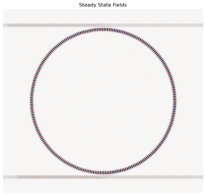
fig = plt.figure(figsize=(12, 8))
ax_field = fig.add_subplot(1, 1, 1)
ax_field.set_title("Steady State Fields")
ax_field.imshow(
np.flipud(np.transpose(eps_data)),
interpolation="spline36",
cmap="binary")
ax_field.imshow(
np.flipud(np.transpose(np.real(ez_data))),
interpolation="spline36",
cmap="RdBu",
alpha=0.9,
)
ax_field.axis("off")
plt.show()
1
Resonance wavelength: 1.5620 μm
This post is licensed under CC BY 4.0 by the author.